An observatory with an outer horizon
Panoptes places massive, autonomous stations in the outer Solar System, beginning with a pair and growing toward a surrounding constellation. Their instruments look both outward, toward other worlds and the Galactic centre, and across the approaches to our own system. The project joins two ambitions: recover spatial information from remote sources, and discover consequential trajectories while there is still time to investigate them.
The Sun supplies one extraordinary observing mode. Beyond roughly 548 astronomical units, rays passing outside its limb can converge along a distant source’s focal line. Panoptes would travel farther into that region, brake substantially, and follow a selected source’s projected image while its direct telescopes continue surveying a much larger sky.
Each station is also an independent observatory: large collecting apertures, sustained nuclear power, local computation, replaceable instruments and robotic service. A first 600-tonne reference makes room for those obligations. Its final shape follows the optics, heat paths and assembly interfaces; a broad instrument body can connect to separately delivered power and propulsion sections.
The surrounding surface marks possible observing positions. The illustrated rays and station locations show relationships, with distances compressed. Each source selects its own line through this geography. Direct telescopes can share a broad field even when their solar-lens targets differ.
Survey
Repeated direct images measure position, brightness, spectrum and change. Cadence and sensitivity determine what enters the catalogue.
Solar-lens imaging
A coronagraph isolates ring light. A moving collector samples an image plane; calibrated reconstruction estimates the source.
Paired observation
Two viewpoints constrain range and verify events. Interferometry adds spatial-frequency measurements when correlation is feasible.
Begin with the isotope after the fire
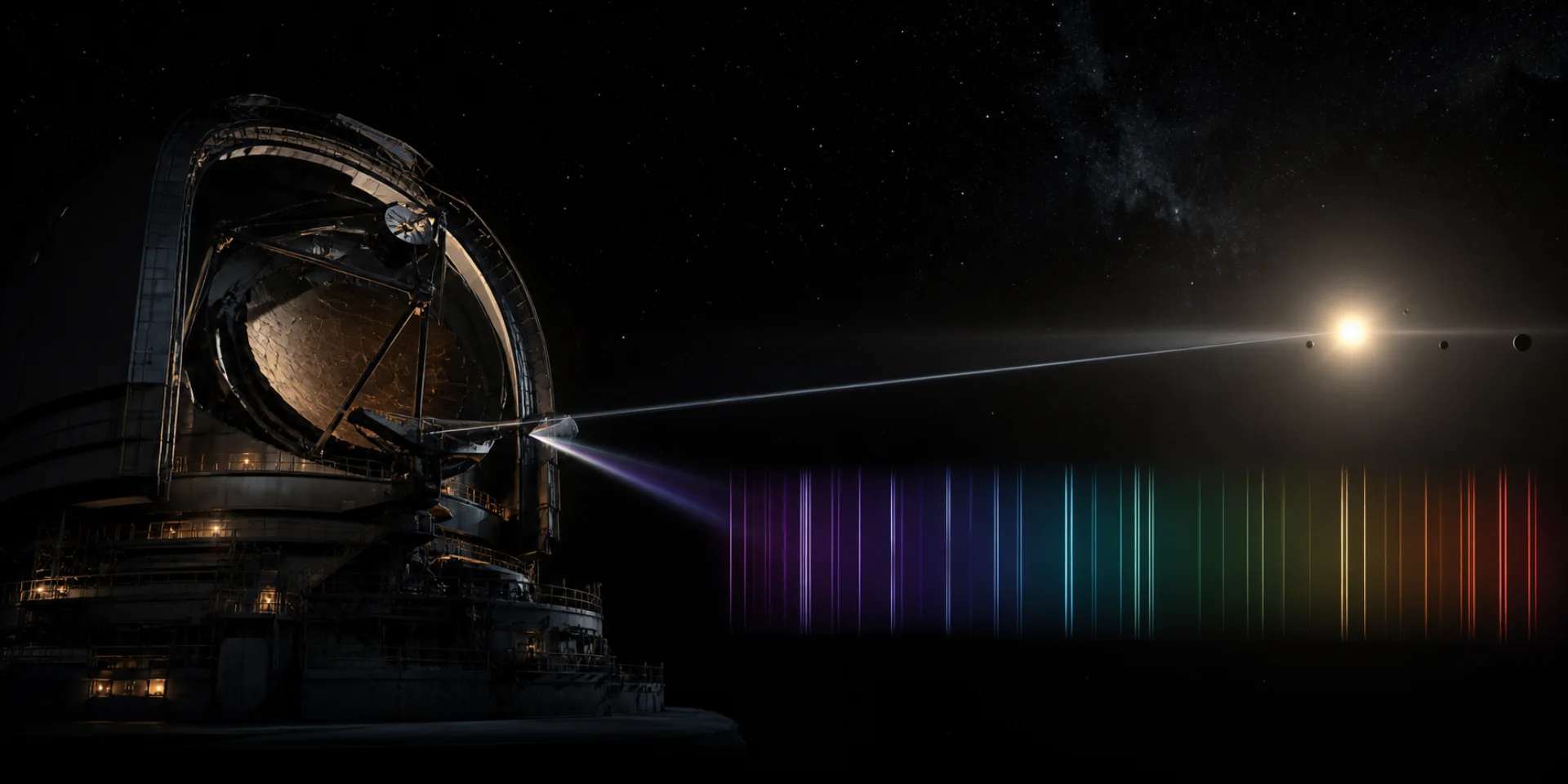
The first stage of Panoptes begins before a station leaves Earth. A nuclear technology can change an isotope inventory that survives long after its short-lived radiation has faded. If some of that material reaches an atmosphere, plume, dust population or debris field, a spectrum might preserve evidence of the activity. The preparatory survey asks which such changes could be measured, which natural processes could imitate them, and which systems deserve the attention of a distant observatory.
This stage supplies a target catalogue and instrument requirements to the larger programme. Laboratory spectroscopy, natural-baseline modelling and archival searches can begin while the observatory architecture develops. A credible anomaly could justify deeper conventional observation and inform a solar-lens target; Panoptes’ planetary imaging and moving-object survey also retain scientific purposes independent of an isotope discovery.
Follow the material all the way to a measurement
A candidate signature needs four connected results. Technology must produce or concentrate it enough to shift a ratio; the useful abundance pattern must persist through decay and chemistry; material must escape into a region accessible to observation; and its spectral information must survive the environment and instrument. Failure at any step breaks the proposed connection between an industrial inventory and an astronomical detection.
Most reactor products remain in fuel, waste, slag, soil or other solids. Persistence alone does not expose them to a telescope. The export model must track how much accessible material exists, its chemical state, dilution and residence time. The measurement model must then distinguish isotope shifts, hyperfine structure or isotopologue bands from elemental abundance, temperature, pressure broadening, winds, rotation, velocity structure and instrument error.
| Candidate | Reason to investigate | Measurement that must be established |
|---|---|---|
| Neodymium-148 | A stable fission product used in reactor burnup accounting; a concrete starting point for an abundance-pattern study. | An export route into observable material and an isotope-sensitive spectrum, compared with natural neodymium and its stellar and chemical history. |
| Ruthenium-99 | A stable endpoint in a different mass chain, useful for comparing refractory transition-metal behaviour. | Whether condensation and retention leave enough accessible material, with nucleosynthesis and ordinary chemistry included in the baseline. |
| Xenon-129 | A noble-gas comparison that changes the transport and retention problem. | An abundance pattern distinguishable from natural, radiogenic and atmospheric-evolution effects; volatility alone does not establish detectability. |
| Barium-135 / 137 | Stable endpoints providing another comparison across production and decay histories. | Useful isotope-sensitive transitions and a joint account of stellar abundances, geology and spectral blending. |
| Lead / mercury | Comparison cases requiring a specific ratio and pathway before being ranked. | Lead must be separated from natural uranium and thorium decay histories; mercury from natural isotope fractionation and chemistry. |
The Atomic Energy Commission’s neodymium-148 burnup method measures material in a laboratory with isotope-dilution mass spectrometry. That establishes a useful terrestrial accounting signature, not remote astronomical sensitivity. The IAEA fission-product reference and evaluated mass-148 datasets support inventory and decay-chain checks. None of the candidates in the table has been selected here as a demonstrated remote technosignature.
The natural baseline includes stellar nucleosynthesis, radiogenic production, cosmic-ray spallation, mass-dependent fractionation, condensation and planetary escape. A technological interpretation must improve a fit that already allows those processes to vary. Measuring an unusual ratio and identifying its cause are separate inferences.
Astronomical isotope spectroscopy has succeeded in favourable settings: Zhang and colleagues detected carbon-13 monoxide in a young super-Jupiter’s atmosphere. That demonstrates access to isotope information and also the importance of natural formation histories. It does not establish sensitivity to terrestrial-scale nuclear residues.
Turn the precursor survey into a target decision
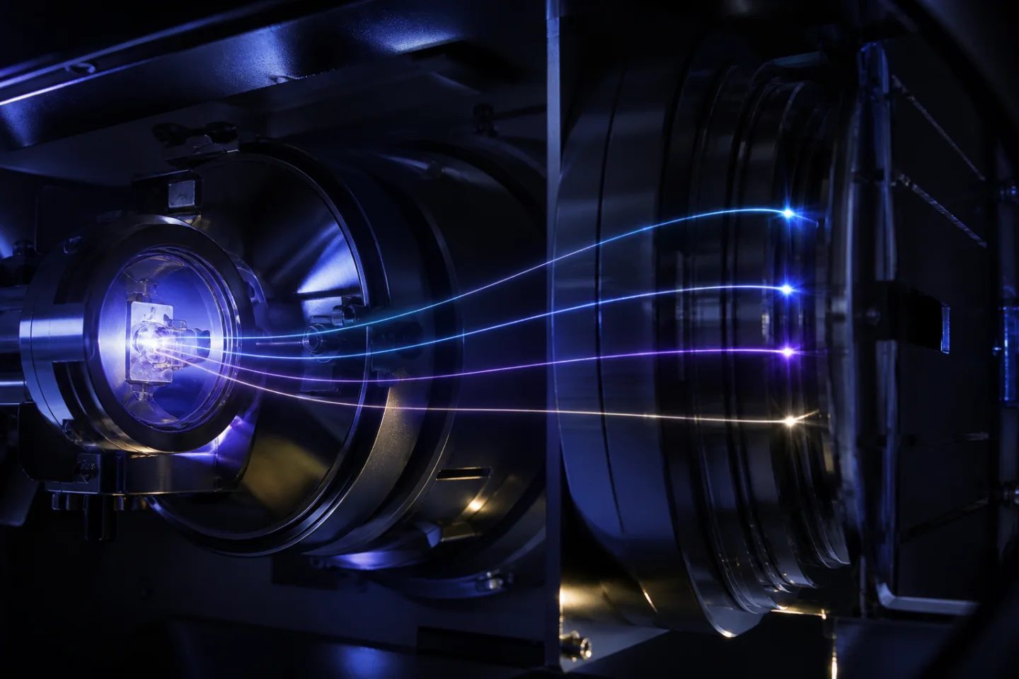
First, compare published nuclear inventories and decay histories with laboratory spectra across candidate chemical states. The purpose is a discriminating abundance pattern and observable transitions. Next, model export, dilution and residence in atmospheres, plumes, dust and debris, beginning with an industrial-Earth analogue whose assumptions can be inspected.
Then pass that model through distance, background, spectral resolution and detector noise. Inject anomalies into realistic spectra and recover them blind against natural alternatives. If the terrestrial analogue disappears, quantify the stronger source, more favourable environment or different instrument that would be needed; that result bounds which systems a search could address.
Search archives with thresholds and candidate-promotion rules specified in advance. A surviving anomaly needs repeated measurements, independent instruments and a fit across multiple useful features. A single blended line cannot carry the interpretation. New telescope time should refine the abundance pattern, environment and natural alternatives before the result enters the dedicated-station target catalogue.
The output is a decision record: candidate transitions and required sensitivity, the sources that survived independent review, and upper limits where the search found nothing. That record informs aperture, wavelength coverage, spectral resolving power, observing cadence and the choice of focal line. If every proposed isotope pathway is inaccessible or naturally explained, this branch returns a quantified null result; the programme does not describe an isotope detector it has failed to justify.
Where the lens becomes usable
The “Einstein bubble” is the geography formed by all possible focal lines around the Sun. For one distant target, the useful station lies on the opposite side of the Sun, beyond the point at which the required rays clear the opaque limb. Moving around the bubble changes the lens target. Moving outward along one line changes ring separation, image scale and the navigation required to keep sampling the same world.
Here b is the ray’s closest distance to the Sun’s centre, rg its gravitational radius, z the station distance and d the source distance. The finite-distance expression matters for nearby targets. At effectively infinite source distance, setting b equal to the solar radius gives the approximately 548-AU boundary.
Geometric monopole lens for a finite source distance. Solar disk and ring use the selected angular field within the ring panel; brightness, ring thickness and instrument suppression are illustrative. The focal boundary uses a source at effectively infinite distance.
At 650 AU the solar radius subtends 1.476 arcseconds; the reference ring lies at 1.607 arcseconds. Only 0.132 arcseconds separates their radii. The instrument must preserve that annulus while suppressing disk light and estimating the extended corona. The ring’s brightness in the drawing is illustrative; geometric clearance alone does not determine signal-to-noise.
An Earth-diameter world at 30 parsecs projects to a 1.338-km image. A one-degree change of target at the station requires approximately 11.3 AU of transverse travel. A constellation therefore buys access to different lines; an individual station cannot switch solar-lens targets as freely as it repoints a direct telescope.
Nearby stations can sample different parts of one extended image or occupy different distances along a line. A widely separated pair ordinarily samples different lens targets, although its direct telescopes may observe the same Galactic-centre field. Source motion, planetary rotation and the Sun’s barycentric movement make lens navigation an active tracking task. The extended-source treatment and focal-line navigation study develop those relationships.
A planet is recovered from overlapping measurements
A detector at one image-plane position receives mixed light from across the source. Rastering the collector changes the mixture; it does not isolate one perfect surface pixel at a time. The forward problem predicts those mixtures from a proposed source. The inverse problem finds a source consistent with the measurements, foreground calibration and assumed response.
An illustrative 16 × 16 raster spans a 1.338-km Earth projection at 650 AU and 30 pc. Cell width is 83.6 m; a 128 × 128 grid would use 10.46 m. Sampling pitch is a coordinate choice, not recovered surface resolution. Measurement footprints overlap.
Envelope surrogate proportional to 1/√(distance² + core²), row-normalized; deterministic noise and nonnegative gradient descent. Omits physical flux, the corona, motion, aperture integration, spectral response and realistic instrument noise. Not an observing-time or resolution forecast.
This small inverse experiment keeps its synthetic source known so that error can be measured. Increasing iterations initially undoes mixing, then increasingly fits the added noise. The response is an envelope surrogate; its core and long tails demonstrate coupling without claiming the photon budget or reconstructed resolution of a physical telescope.
The monochromatic response above is J₀² at 550 nm and 650 AU. Aperture averaging, spectral bandwidth and solar multipoles alter the response used in an actual reconstruction. A sharp point-response core can coexist with a difficult extended-source inverse problem because the wings mix many source locations.
A June 2026 scalar observability benchmark propagates an Earth map through an aperture-averaged model with noise, motion and calibration errors. Its reference 128 × 128 raster at 650 AU and 30 pc uses 1,800 seconds per sample and reports a 232-km resolution proxy after reconstruction. That is about 341 days of integration for one complete raster before overhead. Cloud variability and rotation require registered repeated observations; treating changing measurements as a static planet can fail. These published results supply a more demanding target for a Panoptes instrument study than the illustrative inverse above.
Buy speed near the Sun; buy time at arrival
The departure begins with an inward transfer, followed by a prograde burn at solar perihelion. Burning where the vehicle is already moving rapidly converts a given impulse into a larger change in orbital energy. For a parabolic approach, the ideal result follows directly from the speed before and after that burn:
The reference uses a 0.05-AU perihelion and a 15-km/s impulse. It produces 76.7 km/s of asymptotic outbound speed. A later nuclear braking phase reduces that speed to 15 km/s, retaining 600 tonnes for science, maintenance and reserves. Scrub the flight to inspect position, speed and propellant consumption through its modeled phases.
First-order trajectory trade, not a launch window or full optimal-control solution. Parabolic inbound approach; ideal impulsive injection; analytic solar hyperbola; constant-power, constant-exhaust-speed braking without solar gravity beyond 50 AU. Final mass is held fixed while hardware sensitivity is explored. Electrical efficiency 70%. No extra cruise acceleration.
At 100-km/s effective exhaust speed, the braking reserve is roughly 512 tonnes. Eighteen megawatts of electrical input at 70% jet efficiency produces 252 newtons; braking consumes about 6.4 years and 66 AU. The resulting 650-AU arrival takes about 47.4 years including a five-year allowance for assembly and inward travel. That allowance is not an optimized transfer.
The departure stack is substantially larger. At 900 seconds specific impulse, a 15-km/s impulse requires an ideal stage mass ratio of 5.47. Applied to the fuelled observatory, this already exceeds 6,000 tonnes before the burn. The discarded stage structure, shield, reserves and earlier transport all add mass beyond that lower bound.
The search minimizes braked arrival time over the stated grid: perihelion from the selected minimum to 0.17 AU farther out in 0.005-AU steps, and impulse from 0.5 to 40 km/s in 0.5-km/s steps. Other flight inputs remain fixed. Its mass bound excludes departure-stage dry hardware. At 0.03 AU, incident solar flux reaches about 1.51 MW/m²; the fastest mathematical point must still survive its thermal environment and a finite engine burn.
Arrival is an observing state. Fifteen km/s outward means about 3.16 AU per year, giving a long campaign along a focal line with changing plate scale. Reserves must also support transverse tracking, navigation corrections and fault recovery. Braking to exact heliocentric rest would not produce a stable parking orbit.
The open-exhaust nuclear branch
Direct fission-product propulsion belongs in the mission’s central trade. In this concept, energetic radioactive reaction products escape as part of the useful exhaust. That offers a route to much higher effective exhaust speed than heating a working fluid. The key mission question is how much directed momentum an entire flight engine can deliver per unit of retained vehicle mass, for the required years of operation.
| Route | What leaves the vehicle | Consequence for braking |
|---|---|---|
| Solid-core nuclear thermal | Heated propellant, typically hydrogen; the reactor is intended to retain its fuel. | About 900 s corresponds to 8.83 km/s exhaust. Tens of km/s of braking impose enormous mass ratios. |
| Closed-reactor nuclear electric | Electrically accelerated working propellant. | Higher exhaust speed reduces propellant, while finite electrical power limits thrust. This is the reference branch. |
| Direct fission-product exhaust | Energetic radioactive reaction products in an open-exhaust concept. | A speculative high-exhaust-speed branch. Fuel utilization, collimation, structure, waste heat, shielding and thrust remain unresolved. |
Higher exhaust speed reduces propellant for a specified velocity change. At fixed jet power it also reduces thrust. The following experiment gives this branch its own directed-power input. It does not take that power from the reference observatory’s 20-MWe electrical budget.
Ideal effective exhaust model: constant directed jet power, nonrelativistic exhaust, no engine mass or fuel-utilization model. Jet power is kinetic power in the collimated exhaust; it is distinct from electrical generation and reactor thermal power.
For the illustrated 61.7-km/s velocity reduction and 600-tonne retained mass, an effective 1,000-km/s exhaust needs about 38 tonnes of expelled mass. At 100 MW of directed jet power, ideal thrust is 200 N and the burn lasts about six years. Increasing exhaust speed tenfold greatly reduces expelled mass but extends the burn to roughly six decades at the same power. Engine hardware, fuel that never contributes useful directed exhaust and auxiliary propellant would increase the carried mass.
NASA’s fission-fragment spacecraft study and NIAC fission-fragment concept investigate the propulsion family. Panoptes needs a full-system comparison of usable exhaust, engine mass, lifetime and heat rejection. The open exhaust also determines instrument orientation and operating windows: braking, contamination-sensitive measurements and precision correlation cannot simply run together.
Give the machine a serviceable anatomy
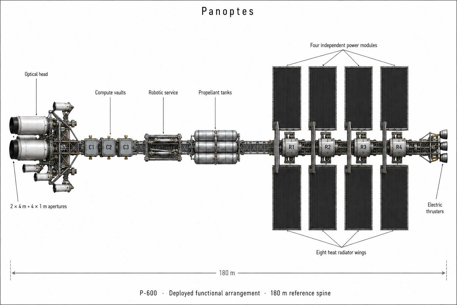
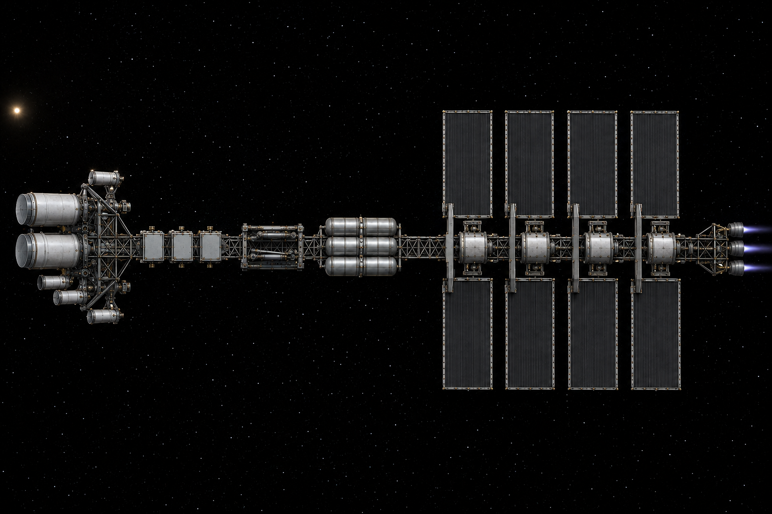
The station’s quiet end gathers light; its power sections reject heat and supply propulsion. Between them sit protected computation, tankage, metrology and routes for robotic maintenance. Separation helps only when cables, cooling loops, shields and structure preserve it. A duplicated instrument still has a common failure if both copies depend on one pump, one power switch or one obstructed service rail.
Functional arrangement, not mechanical dimensions. Cyan follows electrical service; amber follows hot radiator loops. Each power section owns a pair of isolatable hot wings. The optical core is deliberately broad; distances, shield geometry and structural dynamics require engineering closure.
| Allocation | Mass | Included obligation |
|---|---|---|
| Power and principal electric propulsion | 320 t | Four 5-MWe reactors, shields, conversion, distribution, hot radiators and propulsion strings. |
| Optical payload | 60 t | Two 4-m visible/near-IR apertures; four 1-m survey apertures; coronagraphy, spectrometry and separately cooled IR instrumentation. |
| Spine and deployment | 60 t | Structure, mechanisms, isolation and servicing rails. |
| Braking tankage and feed | 30 t | Dry hardware allocation; tank fraction must be recalculated when propellant changes. |
| Compute and storage | 15 t | Three isolated vaults, error-correcting memory, accelerators, recording and recovery hardware. |
| Communication and metrology | 10 t | Two optical terminals, RF fallback, clocks and independent navigation sensors. |
| Robotic service and spares | 15 t | Carriage, manipulators, interchangeable modules and consumable service items. |
| Unallocated margin and retained reserves | 90 t | Mass growth, navigation consumables and remaining design uncertainty. |
| Total after principal braking | 600 t | Braking propellant and discarded transfer hardware are additional. |
The 320-tonne power package implies 16 kg per installed kWe including generation, shields, conversion, hot radiators and principal electric propulsion. That is an aggressive allocation for a long-life space system. Tankage must be rescaled when propellant changes; the 90-tonne reserve cannot cover arbitrary growth in every subsystem simultaneously.
Deliver modules, then connect an observatory
Independent sections use local guidance, docking sensors, attitude control and delivery propulsion or a tug. The instrument body and repeatable power sections arrive as tested assemblies, connect structural and service interfaces, verify isolation, then deploy their working geometry. Four equal power sections average 80 tonnes each before the separately allocated common structure and tankage.
Assembly before perihelion makes one stack to control and shield. Separate solar passes distribute the protection problem across smaller sections but demand a difficult outbound rendezvous. The deployed configuration is not the perihelion configuration: apertures close, wings stow and transfer shielding protects the stack. Delivery engines must clear other modules with their exhaust and cannot be assumed to supply the departure impulse.
Length can separate hot machinery and provide repeated attachment points, while a broad instrument core gives useful equipment volume, collector support and maintenance access. Either geometry must be compared at equal mass, aperture, thermal isolation and failure tolerance.
Serviceability is a physical route: isolate a failed loop, reach its replaceable pump, remove it without disabling the other loops, reconnect, pressure-check and recalibrate. A recovery plan includes a jammed manipulator and the energy and spare parts consumed by the repair.
Twenty electrical megawatts require a much larger heat path
Four 5-MWe modules install 20 MWe. The maximum reference braking state assigns 18 MW to propulsion and 2 MW to services and losses. One failed module reduces propulsion’s allowance to 13 MW. Science operation instead schedules quiet intervals and separately budgets the computing load, cold detectors, metrology and communication.
Stefan–Boltzmann balance for ideal unobstructed two-sided hot radiators. Omits view factors, gradients, damaged panels and piping. Electronics and detector heat must use separate cooler loops; it cannot all be rejected at the hot-loop temperature.
At 25% conversion efficiency, 20 MWe requires 80 MW of reactor heat; 60 MW leaves through the conversion radiators. Eight 20 × 30 m wings provide 4,800 m² of planform. At 600 K and emissivity 0.9, two fully exposed faces radiate about 63.5 MW. That barely accommodates conversion losses; absorbed sunlight, pump work, electrical dissipation, mutual heating and damage margin require additional accounting.
Radiator temperature is a subsystem decision. Computer coolant and infrared detectors cannot simply share a 600-K rejection loop. Cold optics need separate stages and protected views of space. Shadow shields limit direct radiation in selected directions; scattered radiation, structure conduction and pump vibration remain coupled to the instrument layout.
A supercomputer that preserves the evidence
The station processes measurements locally because raw acquisition can exceed the link by orders of magnitude. Four hypothetical gigapixel cameras recording 16-bit frames every second produce 64 Gbit/s, or 691 TB per day. An uninterrupted 1-Mbit/s downlink carries 10.8 GB per day. Selecting one frame in a thousand still leaves roughly 64 times too much data for that link.
Four cameras, 16 bits per pixel; no compression overhead, calibration planes or link outages. Downlink rate is a scenario input, not an optical-link budget. Intensity frames do not preserve the optical electric field phase.
The reduction pipeline calibrates detector effects, removes predictable background, searches candidate tracks, compares independent reductions and packages follow-up requests. A rolling buffer keeps raw event cutouts, timing, calibration and nearby negative examples. Routine sky products can be compressed aggressively; unexpected results need enough original evidence to support a different interpretation.
At 650 AU, Earth’s answer arrives about 7.5 days after a question leaves the observatory, even before people deliberate. Three computing vaults divide active processing, independent checking and a recoverable spare. A conservative safety controller limits science workloads, protects power and cooling, and can return to an immutable recovery image. Identical algorithms running three times do not independently validate a discovery.
Intensity frames contain measured brightness, not the optical field phase. More storage and faster processors cannot reconstruct an unrecorded phase reference. The correlation architecture must therefore be selected at the detector and timing level, before deciding which stream the supercomputer will reduce.
What a second station actually adds
A second viewpoint immediately adds independent confirmation and parallax. Direct interferometry asks a further question: can the stations measure a useful correlation in received light? Its angular scale follows the projected separation perpendicular to the target, λ / B⊥. Collection area remains the sum of the real apertures, and photon statistics still determine whether that spatial information is measurable.
Direct, unlensed telescopes. Two 4-m apertures, 30% throughput; 1,000-second photon-count example per aperture, AB flux density approximately flat within the selected channel. Fringe panel is an ideal one-dimensional two-aperture response, not an image recovery or a sensitivity forecast. Angular sky extent is schematic.
The spatial-frequency panel below changes the number of sampled orientations. A single pair at one instant produces parallel ambiguity bands. Additional orientations localize the response and alter sidelobes. The map is a normalized dirty beam from equal, noiseless samples: it shows the array’s response to a point source, not a recovered astronomical image.
Equal-length projected baselines with conjugate samples. Map axes are angular offset in units of λ/B; zero-noise, equal weights and a static source. Orientations require array motion over time or additional stations.
For 550-nm light, 55 nm of residual optical path is a tenth of a cycle. A narrower spectral channel lengthens the coherence envelope but reduces photons in that channel. A moving target may cross the formal angular scale faster than the necessary integration; this is why photon count, delay, path stability and motion appear next to the baseline calculation.
| Method | What must survive | Unresolved requirement |
|---|---|---|
| Direct amplitude combination | The received optical fields and their relative path. | Transport loss, delay compensation, acquisition, nanometre-scale residual path and formation metrology. |
| Optical heterodyne recording | A measured field relative to a local oscillator. | Oscillator transfer, phase reference, detector bandwidth, channelization and quantum-noise sensitivity to faint targets. |
| Intensity correlation | Time-resolved photon-intensity fluctuations. | Timing, photon statistics, useful correlation contrast and enough spatial samples to constrain a source. |
MAGIC observations demonstrate optical intensity interferometry on bright stars. That method relaxes optical phase-path requirements while retaining demanding photon and timing requirements. Additional stations provide more baselines; amplitude interferometers with three or more stations can also form closure-phase information.
A common Galactic-centre field
At 8,000 parsecs, a one-AU projected baseline gives a formal 550-nm scale near 900 m. Measuring structure on that scale still requires correlated source photons, a delay model and adequate sampling before the source changes. Travelling 650 AU does not leave the Galactic dust behind; visible and near-infrared views of the centre show why extinction, wavelength and source confusion belong in target selection.
Combining two solar-lens collectors is a separate propagation problem. Both apertures sample a structured lensed wavefield that depends on the finite source, Sun, foreground and collector position. The useful baseline and mutual coherence must be derived from that field. Independent reconstructions may prove more useful for some arrangements; multiplying direct-aperture resolution by solar-lens amplification does not establish a combined instrument.
Discover a trajectory, then measure its consequence
The defence task begins with a track: repeated positions and times, uncertainty, a distance constraint and a trajectory fit. Speed and size determine an energy scale only after specifying the encounter frame. In the nonrelativistic limit, equal-energy bodies at equal density obey D ∝ v−2/3. A body ten times faster can be about 4.6 times smaller at the same kinetic energy.
Spherical body at 3,000 kg/m³; relativistic kinetic energy; constant rectilinear remaining distance. Heating assumes complete capture of pure hydrogen kinetic energy, redistributed over the entire body and radiated with emissivity 0.9. It omits solar heating, dust impacts, ablation, plasma and incomplete energy deposition. Reflected magnitude assumes albedo .05 and full phase, and is a separate estimate.
Encounter speed sets the kinetic energy; closing speed sets straight-line time remaining; gas-relative speed sets the heating estimate. These are independent controls because they describe different relative motions. Energy equivalence alone does not predict damage: composition, fragmentation, geometry and coupling to the atmosphere or surface determine the outcome.
Speed does not supply visible luminosity without an interaction. At 0.1c through hydrogen at 0.1 atom/cm³, the ideal complete-capture, whole-surface estimate gives only about 58 K before solar heating, peaking in the far infrared. Partial deposition, dust impacts and an emitting wake change the signal. A bright cloud can help discovery while displacing the measured centre of light from the solid body.
Recover motion without painting it into the evidence
The exposure sequence below uses fixed-seed noise and a source injected with the calculated single-exposure significance. The marker shows the known injection position for explanation. It does not establish a detection. Fainter settings blend into the background; increasing exposure adds photons but also lengthens the trail.
One 1-m aperture at 550 nm, 100-nm band, throughput .3; 1-arcsec samples and reference point footprint; AB sky surface brightness 23 mag/arcsec²; 3-electron read noise. White-noise estimate, no confusion or instrument systematics. Three fixed-seed Gaussian residual fields use a sampled Gaussian/trail template, normalized to the analytic aperture-sum S/N. Display samples may aggregate angular area and are not native pixels. Known injection markers are explanatory; this is not a recovered trajectory. Four survey cameras, 50% net observing duty, no field overlap in the optimistic sky-coverage calculation.
Cloud size holds total source flux fixed here. Spreading that light across more detector samples increases background noise. A physical cloud might also add emission or scattering; that requires a separate luminosity model. Likewise, a track selected after searching millions of possible velocities needs a trials correction before its significance becomes a false-alarm probability.
A usable warning is shorter than the geometric travel time: photons must reach the station, another epoch must constrain motion, and a message must reach Earth. Close or extremely fast events can outrun that process. The two stations must preserve their individual astrometry and uncertainty, then update a joint trajectory with enough evidence to expose a bad association.
Discovery
Inject objects into realistic backgrounds across brightness, velocity, cloud size and observing direction. Measure recovery and false alarms.
Association
Connect epochs and viewpoints with a trajectory hypothesis. Fit uncertainty and retain alternative tracks until evidence separates them.
Follow-up
Reobserve, obtain spectra and refine range. Reserve raw cutouts and calibration so independent reductions can challenge the result.
At 650 AU, sunlight is about 1/422,500 as intense as at Earth. Cold, dark bodies can be difficult reflected-light targets even with a remote vantage. Thermal infrared belongs alongside visible survey, but the cold interstellar population differs from the solar-heated targets of NEO Surveyor. A surrounding watch must be evaluated against nearer telescopes using the same encounter catalogue and resources.
An autonomous watch with a testable programme
A possible interstellar traveler belongs among the explanations to investigate. Non-gravitational acceleration, unusual spectra or repeating time structure can motivate another observation; natural outgassing, radiation pressure, source confusion and detector faults must remain in the comparison. The station’s authority is to secure itself, collect evidence, revise its observations and communicate an accountable result.
The precursor isotope survey establishes candidate targets and measurement requirements. The next mission study connects those requirements to the instrument and vehicle calculations. Propagate a moving source through the solar lens into a finite aperture and calibrated detector; recover a held-out spatial property. Inject a synthetic encounter population into the direct survey; measure discovery and trajectory recovery including delayed communication. Close a propulsion branch against its complete engine, propellant, power and radiator masses. Demonstrate useful science while a failed module is isolated and serviced.
These experiments determine which capability earns each tonne and each year of travel. The reference gives them a common observatory to interrogate: an outer-system pair, a substantial retained machine, solar-Oberth departure, significant nuclear braking, and enough local intelligence and maintenance capacity to remain useful after Earth is days away by light.
The model notes document the approximations, and the calculation source exposes the numerical relations used here. The diagrams are authored schematics. Spacecraft images remain packaging studies; the spectroscopy images are concept art.