Active research · learned geometry

The M-layer
experiment

We began with a layer that carried one beautiful geometry. We ended with a harder question: can a network learn which geometry the observations permit before it commits to one?

The question now

Can a pointwise model turn the relations among observations into a reusable connection—without being handed the coordinate system, the recurrence, or the geometry it is supposed to discover?

The initiating mistake

A geometry can win for the wrong reason.

The original M-layer used a global matrix exponential. That is a formidable prior when the target is genuinely group-like: rotations, oscillations, flows, and nilpotent polynomial structure all have natural homes there. The same elegance becomes an epistemic trap when the task is localized, branching, piecewise, or governed by a frame that changes from place to place.

If a Fourier map wins a periodic problem, or a matrix exponential wins a rotational one, it may have discovered nothing. We may simply have put the answer in the surface of the model. The experiment therefore changed direction. “M-layer” now names the provocation, not the surviving architecture.

The replacement criterion was stricter: preserve an ordinary affine path; let the current activation construct a private hypothesis about its own local geometry; re-read the same activation through that hypothesis; and make every comparison against a same-budget ordinary MLP.

The mechanism that survived

Self-context: let the activation propose its own chart.

For an authentic hidden activation x, the layer keeps a fixed bank of unprivileged projection frames P_d. It does not pick a frame globally. A learned positive-semidefinite metric M(x) measures the projected evidence at this particular activation, and a soft allocation assigns responsibility across the bank.

Projectp_d = P_dx
Several low-rank views observe the same authentic state.
MeasureM(x) = A(x)A(x)^T / r
The activation supplies its own local metric.
Allocatew_d = softmax(response − cost / τ)
Chart choice stays continuous; no hard atlas label is supplied.
Liftc(x) = Σ_d w_dP_d^Tp_d / r
The selected views become a contextual displacement.
Re-readx′ = x + γ · rms(x)c(x)/rms(c)
The layer recomputes its chart from an anchored reinterpretation of the same state.

Distilled from ML_experiment/models.pyPyTorch

def self_context(x):
    factor = metric_net(x).view(B, rank, rank)
    metric = factor @ factor.transpose(1, 2) / rank

    projected = einsum("dri,bi->bdr", primitive_frames, x)
    cost = einsum("bdr,brs,bds->bd", projected, metric, projected)
    weight = softmax(response(projected, cost) - normalize(cost), dim=1)

    context = einsum("bd,bdr,dri->bi", weight, projected,
                     primitive_frames) / rank
    context = context * rms(x).detach() / rms(context)

    # The proposal changes the chart, not the authentic residual path.
    chart_x = x + context_strength * context
    _, projected, weight = allocate(chart_x)
    pooled = einsum("bd,bdr->br", weight, projected)

    return affine(x) + softplus(scale) * (pooled @ shared)

This is the conceptual core, with diagnostic and experimental branches removed. The implementation anchors refinement to x; repeated context does not accumulate as an uncontrolled state drift.

It can abstain.

The affine path remains intact. Structured correction is residual, learned, and scale-controlled.

It is conditional.

Two activations can allocate the same primitive views differently. There is no single geometry imposed on the whole task.

It is continuous.

Soft allocation avoids brittle chart switches and lets backpropagation redistribute responsibility.

It is still pointwise.

The context comes from one activation. It does not remember the observation set or infer a recurrence between samples. This limitation matters.

What the batteries actually say

Broad competence beat a sequence of beautiful exceptions.

In the first exact-budget 22-problem confirmation, self-context raised mean held-out score from .610 for an ordinary LELU MLP to .704, and learning-curve area from .744 to .857. It was about eleven times slower, which is not a footnote: the baseline earns structure by doing substantially more work per activation.

Later batteries found models with higher mean endpoints. Continuous frame flow, for example, reached .679 held-out versus self-context’s .665 on a 23-problem width-24 battery. It also cost 3.32 times the wall time and concentrated its advantage in a few geometries. A later width-38 battery narrowed the mean gap to .676 versus .672 while keeping roughly the same fourfold compute separation. That is why “best approach” here means the best current default, not the largest aggregate rounded to three decimals.

Mechanism	Held-out	Learning AUC	Seconds / task	What the average hides
Ordinary LELU MLP	.585	.731	.40	Cheap, honest control; misses much of the acquired structure.
Self-context	.672	.852	4.29	Strongest broad default; still fails genuine continuation.
Continuous frame flow	.676	.864	16.56	Radial and changing-frame specialist; expensive and task-sensitive.
Shallow odd cubic	.510	.587	.40	Perfect on one high-rank spiral because the task exposes an odd invariant.

Two-seed, 23-task, 500-step battery for the common rows above. Parameter counts differ for the deliberately tiny odd-cubic control; the other comparisons are budget-matched within task.

The failure we keep

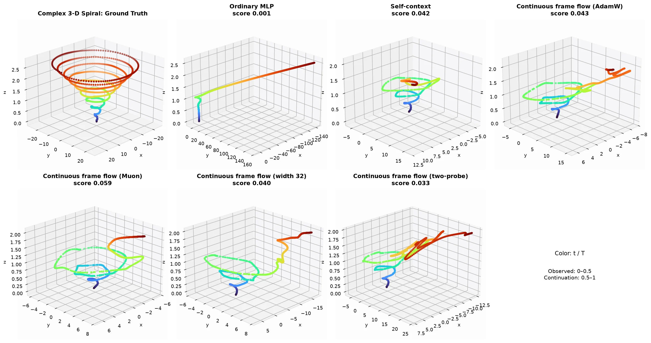
Fitting the observed curve is not learning its law of motion.

The spatial 3-D spiral makes the distinction visible. Self-context and continuous frame flow recover far more of the observed segment than the ordinary MLP. Every displayed model still departs from the true continuation after the evidence boundary. More width does not cure it. More optimization can improve the fitted partition and leave the unseen region at chance.

The model has learned what goes with what here. It has not learned the generator that says what comes next.

Seven 3-D plots compare the true expanding spiral with an ordinary MLP, self-context, and continuous-frame-flow variants. All learned curves diverge during the unseen half. — **Complex 3-D spiral.** Color runs from observed blue-green to unseen orange-red. Scores remain low because the outer half is a continuation test, not interpolation disguised as a test set.

What we tried after self-context

Every extension revealed a real operator—and the boundary of that operator.

Harder allocation, repeated context, entropy gates

Hard allocation accelerated acquisition on 21 of 22 early problems. A second anchored reread mostly added cost. Asking for more context when allocation was uncertain sounded principled and performed worse: low entropy can itself be evidence.

Survived: temperature as a training knob, not a new law.

Curvature shells and continuous frame flow

Antithetic probes measure how the selected frame bends. This produced the clearest radial-stripe and chirp gains, and a decisive high-rank N-D improvement. It also damaged localized steps and could cost three to four times self-context.

Survived: a specialist for transported geometry.

Relational response, learned cones, operator spheres

Richer response heads sharpened chart ownership but often committed too early. The operator sphere correctly learned when a task wanted odd relation, tangent, or curvature; mixing those operators forced one to steal energy from another.

Survived: operator identification, not operator composition.

Odd cubics and bispectral sketches

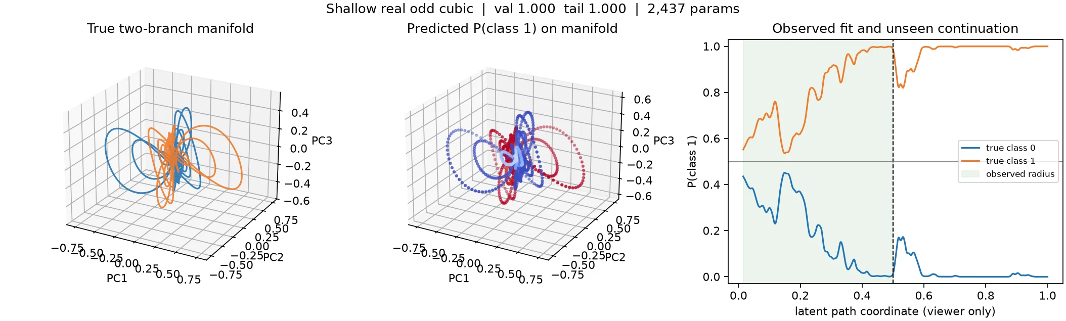
A shallow odd cubic reached 1.000 on the high-rank 16-D spiral. The triumph was diagnostic: the two branches were antipodes, so a third-order product exposed a stable sign. The same model failed the low-rank spiral and the broad battery.

Survived: an excellent cheap invariant detector.

Hermite cells, support measures, zonotopes

Support-stratified sampling repaired a sparse sine whose final observed period carried only 1/96 of the first period’s gradient mass. Three self-context branches selected by a held-out witness removed a bad optimization basin. Neither result continued five unseen periods.

Survived: reconstruction measure is not recurrence.

Commuting scalar charts

On periodic N-D, self-context manufactured mixed curvature where the truth had eight fixed independent axes. A scalar chart bank reached .994 R² with no Fourier features. Its identity-preserving initialization already began in the right frame; random-frame acquisition remained unstable.

Survived: the representation is solved; frame discovery is not.

A spectacular exception, audited

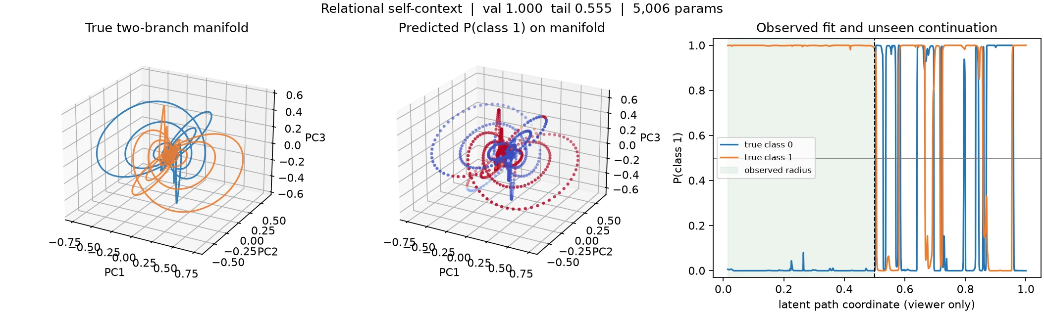
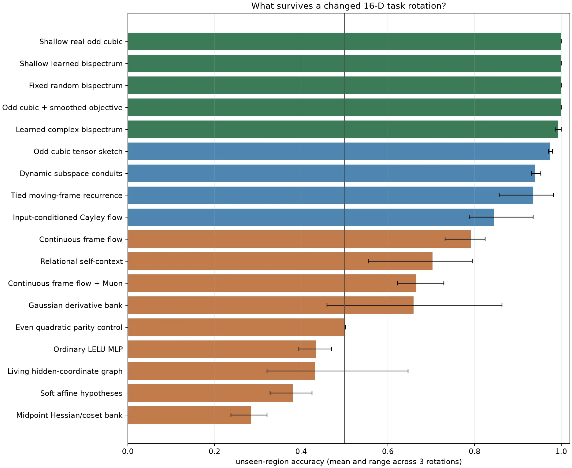
The odd cubic found the answer. Then we changed the question.

On one high-rank spiral rotation, self-context fit the observed half perfectly and continued irregularly. A tiny shallow odd-cubic model continued perfectly. Across changed task rotations it remained extraordinary—but the parity control exposed why: the generator supplied an antipodal relation that any odd third-order statistic could preserve.

This is useful science precisely because it narrows the claim. The model detected algebraic coherence. It did not learn a universal spiral.

Self-context fits a high-rank spiral wall perfectly on observed support but alternates irregularly in the unseen half. — **Self-context.** Perfect observed fit; tail .555 on this seed.

A shallow odd-cubic model cleanly separates both branches of the high-rank spiral wall through the unseen half. — **Shallow odd cubic.** Tail 1.000—because odd parity is the exposed invariant.

Horizontal bars compare unseen-region accuracy across changed 16-dimensional task rotations. Odd-cubic and bispectral methods lead, self-context is in the middle, and the ordinary MLP is below chance. — Mean and range across three changed 16-D rotations. The result survives rotation, but not a change in the underlying antipodal construction.

The exposed boundary

The missing mechanism lives between observations.

Self-context is a private thought inside one forward pass. It can learn that a point resembles a local chart state. It cannot, by itself, retain a hypothesis about how chart states transform across an observation set. Curvature probes still query a pointwise field. Hermite cells improve local reconstruction. Witnessed optimizers select better basins. None of them creates episode memory.

The next credible step is therefore not another response MLP and not a larger mixture of every successful branch. It is a set-conditioned connection: infer a bounded bank of transition hypotheses from relations among observed samples; use evidence to eliminate or merge them; and transport a new query through the surviving state. Sparse sine is the scalar falsifier. Low-rank N-D spiral is its projective analogue.

That proposal is intentionally harder than adding a Fourier feature. It asks the model to learn not only a chart, but what remains invariant when the chart moves.

Research ledger

Nothing here depends on a single flattering score.

The BFFT checkpoint retains model code, raw fits, paired summaries, fitted-function probes, interactive reports, and negative branches. The public claim can be audited against the experiment that produced it.

00Optimizer observation experiment 01Hypothesis and constraints 02Self-context implementation 0323-task response battery 04Sparse support diagnosis 05Commuting-chart exception 06Fusion failures