01 · Introduction
Interpolation begins with missing variation.
Samples record values. Their forward differences also record an ordered sequence of rising, level, and falling intervals. Filling the space between samples therefore chooses a derivative-sign topology as well as a set of intermediate values.
Nearest-neighbor and multilinear rules preserve a narrow range of behavior by discarding resolved shape. Cubic and windowed-sinc kernels recover shape with signed lobes that can insert extra extrema near transitions. Passband fidelity and output range leave that added rise–fall structure largely invisible.
CONV makes the missing state explicit. The endpoint difference supplies conserved current mass. The sequence of secant signs supplies an ordered lineage. A high-order local model proposes how to distribute the current inside each cell, and exact projection changes only the components that conflict with the recorded lineage.
Shape-preserving cubic and quintic splines already constrain monotone intervals. CONV carries the order of transitions across the whole sampled line and permits a witnessed transition to move into a nearby current slot selected by least disagreement. The resulting convex fibre joins endpoint conservation, deterministic admission, and the variation-diminishing proof in one finite operator.
Values say where the curve must pass. Signed current says which turns the curve is allowed to contain.
02 · Interpolation requirements
Six requirements force one representation.
These properties jointly determine the quintic degree, the current coordinates, the admission rule, and the lifting state. Each later formula exists to satisfy this set together.
Observation consistency
𝒯s refines the grid; Ds selects every sth site. Their composition is the identity. Every observed pixel therefore retains the status of evidence throughout synthesis.
03 · Compact two-jet
Accuracy enters before constraint.
CONV begins with a five-point estimate of the first and second derivatives. On a smooth, unit-spaced interior line, both estimates are fourth-order accurate. Centered and one-sided closures handle the two ends from observed samples alone. The proposal therefore contains resolved local shape before admission examines its sign structure.
Interior jet
The two-jet supplies local geometric accuracy. The lineage supplies admissible derivative-sign order. Their separation preserves the full proposal wherever its current already agrees with the sampled record.
The jet becomes six quintic Bézier controls in each cell. Their five consecutive differences form the proposed differential current ai. The five currents already add to the cell’s endpoint difference. Admission changes their distribution only when their signs contradict the ordered record, so the compact jet remains active across the resolved smooth regime.
04 · Ordered lineage and convex admission
The samples supply an ordered sign lineage.
The coarse secants δi = yi+1 − yi create a sequence of plus, zero, and minus evidence. Zero runs inherit the last nonzero sign, with the first future sign seeding an initial zero run. Each observed sign transition receives one ordered boundary. A local least-disagreement rule places that boundary among nearby control currents without allowing transitions to cross.
Signed mass fibre
The sign sequence and mass constraint define a closed convex slice of an orthant. Euclidean projection supplies one nearest admitted current. Because all feasible points have the same total mass, the correction can relocate within-cell motion without changing the observed endpoint difference.
05 · Synthesis
Bernstein synthesis turns admitted current into a curve.
Cumulative sums of the admitted current recover six quintic Bézier controls from the left sample. The nonnegative Bernstein basis then evaluates the curve. Total positivity carries the discrete sign-order bound into the continuous derivative: the synthesized segment cannot oscillate more often than its admitted current sequence.
Quintic Bernstein synthesis
Drag the phase. De Casteljau evaluation follows the control polygon while the endpoints remain fixed.
06 · Scale-global reduction
Shrinking integrates the geometry already constructed.
A smaller image asks for the average content of each target pixel. The admitted CONV profile already describes the source continuously, so reduction integrates that profile across the target grid’s clipped Voronoi basins.
For target coordinate xr = r(N−1)/(M−1), the basin reaches halfway toward its neighboring target coordinates and clips to the source domain at the two ends. The reduced sample is the basin average. Because each source-cell profile is quintic, three-point Gauss–Legendre quadrature is exact on every cell fragment. The browser compiles those fragment integrals once per axis and reuses them for every scanline.
Basin restriction
Every output value accounts for the entire interval it represents. Constants remain exact, total integrated content is conserved, and high-frequency alternation is averaged before it can alias into the smaller grid.
In two dimensions, synthesis is horizontal then vertical, so matched reduction completes the factors in reverse order: vertical basins first, horizontal basins second. A mixed resize completes every reducing factor before every enlarging factor. This is the transport rule implemented in the instrument above.
07 · Cartesian construction
Images inherit one ledger per Cartesian factor.
CONV applies the same componentwise operator across one image axis, reaches a synchronization barrier, then analyzes and synthesizes the other axis. The declared order belongs to the operator. Permuting the data axes together with that order produces the correspondingly permuted result.
The formal two-dimensional construction evaluates both factor orders. A source-conditioned Riemannian action transports the nodal order coordinate, and a structure-tensor admission blends the two results convexly. At source nodes, the apparent all-source chart bank collapses to a Kronecker trace. CONV* extends that trace with the unique cellwise bilinear coordinate, so the only two-dimensional compilation defect is the coordinate error multiplied by the disagreement between the two factor orders.
The action is well-defined on the closed source rectangle. Its continuous positive-definite metric makes the resulting distance finite, continuous, and bi-Lipschitz equivalent to ordinary distance; a shortest path is attained. If several shortest paths tie, admission remains single-valued because it uses their common minimum length rather than choosing a path.
Ordered factor composition
Each order contains a full intermediate-field barrier. Their convex admission is exact wherever the two orders commute, including constant and affine coordinate fields. The browser resizer exposes the compact ordered transport core directly; the paper develops and audits the full Eikonal order blend separately.
The blend adds one derivative term. Convex admission keeps the final value between the two factor-order candidates. Along a line, a varying admission weight also contributes θ′(B−A). The unconditional sign-pair theorem therefore applies to each declared Cartesian composition; the linewise sign topology of the spatial blend follows the paper’s exact derivative criterion.
08 · Analytical properties
The main theorem controls topology.
Ringing here means an added pair of derivative-sign transitions along an admitted Cartesian factor. This definition separates unwitnessed oscillation from amplitude overshoot and from the ordinary movement of an existing extremum between sample nodes.
Cardinality and commutation. Nested coarse samples are exact, and fine differences block-sum to their coarse current.
Affine reproduction. The compact jet recovers an affine line exactly; admission has nothing to change.
Factorwise ringing incapability. Along each admitted Cartesian factor, the synthesized derivative has no more sign changes than the sampled differences.
Grid-size-independent bounds. Pointwise and mean-square error depend on fixed local constants and source error, not on the number of lattice sites.
For each fixed transverse coordinate and each admitted factor, total positivity carries the ordered coefficient bound into the continuous derivative.
Scope of the theorem: along each admitted Cartesian factor, CONV cannot create an alternating rise–fall or fall–rise pair absent from the sampled differences. An existing extremum may move between nodes, and a general path across the tensor-product surface has no corresponding theorem. The guarantee is exactly the one used by ordered grid transfer: every factor inherits its turns from recorded factor currents.
09 · Restriction and matched multiresolution
The same current state survives a change of scale.
Dyadic raster analysis treats each adjacent fine pair as a cell. Its parent is the positive average, which annihilates the Nyquist component exactly; its complementary coordinate is the centered child moment. CONV predicts the admissible moment from the coarse averages, and the difference between that prediction and the true child moment becomes the lifting residual.
Zero-residual synthesis preserves cell mass and transported sign variation while discarding unpredicted fine structure. Restoring the residual moments reconstructs every fine value exactly in arithmetic. In two dimensions, one block mean and horizontal, vertical, and mixed residual moments account for every scalar degree of freedom.
Analysis / synthesis pair
10 · Synthetic evaluation
Admission removes topology errors without blunting the jet.
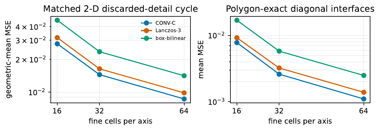
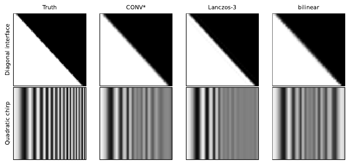
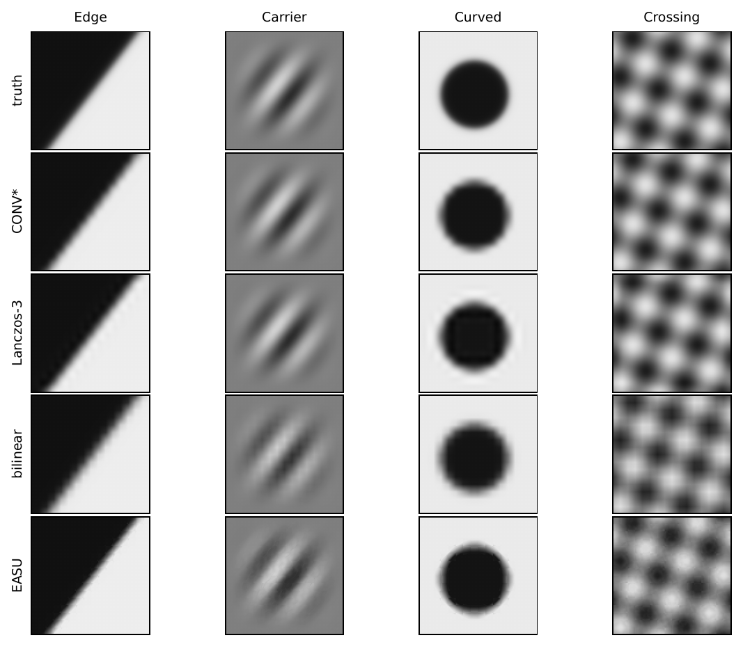
The evaluation uses direct target values from declared closed-form carriers, edges, bumps, chirps, radial transitions, and crossing fields. Separate censuses measure point fidelity, sign topology, and matched analysis/synthesis behavior.
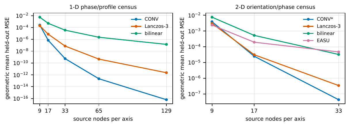
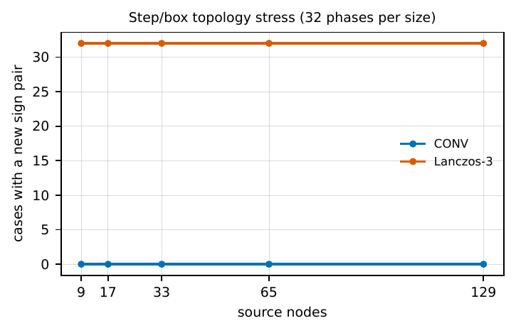
The decisive ablation keeps the stencils, quintic controls, Cartesian order, and evaluator while removing only current admission. The raw proposal adds sign changes in all 160 step and box cases; admitted CONV adds none. Across every reported grid, CONV also has slightly lower aggregate MSE than the raw proposal and converges to the same resolved-field behavior. The proposal remains intact on resolved smooth cells; admission activates where a conflicting current would create a topology error.
At nine source nodes, several analytic populations remain underresolved and Lanczos-3 retains the aggregate advantage. Once the census resolves, the compact jet’s approximation order dominates: CONV wins every one-dimensional case at 129 nodes and gives lower geometric-mean error on the reported 17 × 17 and 33 × 33 two-dimensional grids.
| Source nodes | 1-D W–L | 1-D ratio | 2-D W–L | 2-D ratio |
|---|---|---|---|---|
| 9 | 28–28 | 1.247 | 9–19 | 1.277 |
| 17 | 36–20 | 0.0929 | 19–9 | 0.800 |
| 33 | 44–12 | 0.00751 | 14–14 | 0.126 |
| 65 | 52–4 | 0.000481 | — | — |
| 129 | 56–0 | 0.0000275 | — | — |
11 · Compiled execution
Most of the proof compiles into a compact image operator.
At a fixed integer scale, the formal stages reduce to a compact FIR current bank, a segmented sign scan, exact five-value admission, and a polyphase dot product. CONV* names this compiled schedule. Every reduction is algebraic, and its measured output agrees with the formal operator at binary64 rounding scale. The lineage scan remains because a zero run may inherit its sign from a witness arbitrarily far away.
Twofold midpoint
The Bézier controls never need to be stored. At fixed scale, the cumulative Bernstein weights become a small phase matrix.
Five breakpoint intervals replace 31 face tests.
The new reduction follows the KKT conditions. For ledger sign σj, each admitted current is a clipped shift of its proposal: positive slots use max(0, aj − λ) and negative slots use min(0, aj − λ). Their sum is continuous, nonincreasing, and piecewise affine in λ, with only five breakpoints. Sorting those values exposes at most six affine intervals; the root inside the valid interval returns the same unique projection as the 31-face search.
The implication is executable: the browser’s WebAssembly kernel performs a five-value sort, one scalar root, and five clips per component. Exact admission avoids constructing and scoring every nonempty face.
Lineage has an exact scan schedule.
Zero-sign inheritance is a seeded prefix propagation. Transition costs split into a prefix conflict sum and a suffix conflict sum. Only runs of adjacent coarse transitions retain boundary dependence, and each transition in such a run is a deterministic map over nine possible offsets. Associative composition permits an exact parallel prefix schedule while retaining the first-minimum tie rule.
A barrier remains between Cartesian factors because the second factor analyzes the nonlinear field synthesized by the first. Tiled transposition can make both passes contiguous; removing the barrier would change the operator.
These reductions specify the exact work schedule. Actual throughput still depends on the target architecture: scans and local scalar admission compete with intermediate-factor traffic, so the algebra alone supplies no universal performance ordering.
Arbitrary targets compile too.
Integer refinement repeats a small phase bank. An arbitrary target has a finite coordinate plan: one source cell and five cumulative Bernstein weights for each output site. Reduction has a similarly finite basin plan. The exact Gauss integrals collapse into one anchor coefficient and five current coefficients for each source-cell fragment crossed by a target basin.
The browser compiles either plan once per axis, then reuses it across every row or column. The hot loop becomes coefficient application over admitted current. WebAssembly owns the image-sized intermediate, keeps the work off the main thread, and remains the default backend whenever the browser exposes it.
12 · Inversion and method boundary
CONV is one geometric state with several exact views.
The admitted current defines a continuous source-cell profile for arbitrary endpoint-aligned interpolation. Basin integration restricts that profile to a smaller raster. At dyadic scale, positive averages and residual centered moments turn it into a conservative lifting transform. Repeated phases compile into a polyphase bank, while arbitrary targets compile into a finite coordinate plan.
Wavelet lifting establishes the analysis–prediction–detail principle, while shape-preserving splines establish constrained polynomial reconstruction. CONV joins those lines through transported differential current: the predictor used to create new samples is also the predictor used to explain and exactly recover fine-scale variation.
The browser realizes the ordered transport core in SIMD WebAssembly, processes the two Cartesian factors in cancellable chunks, and downloads the result as PNG. The formal Eikonal order blend, conservative lifting state, and compact browser transport are clearly separated implementations over the same admitted-current geometry.
13 · Selected references
Lineage of the work.
- C. E. Shannon, “Communication in the presence of noise,” Proceedings of the IRE, 1949.
- C. Lanczos, Applied Analysis, 1956.
- R. G. Keys, “Cubic convolution interpolation for digital image processing,” IEEE Transactions on Acoustics, Speech, and Signal Processing, 1981.
- F. N. Fritsch and R. E. Carlson, “Monotone piecewise cubic interpolation,” SIAM Journal on Numerical Analysis, 1980.
- J. M. Hyman, “Accurate monotonicity preserving cubic interpolation,” SIAM Journal on Scientific and Statistical Computing, 1983.
- P. Costantini, “Co-monotone interpolating splines of arbitrary degree—a local approach,” SIAM Journal on Scientific and Statistical Computing, 1987.
- R. Dougherty, A. Edelman, and J. M. Hyman, “Nonnegativity-, monotonicity-, or convexity-preserving cubic and quintic Hermite interpolation,” Mathematics of Computation, 1989.
- T. Lux, L. T. Watson, T. Chang, and W. Thacker, “Algorithm 1031: MQSI—monotone quintic spline interpolation,” ACM Transactions on Mathematical Software, 2023.
- S. Karlin, Total Positivity, 1968; A. Pinkus, Totally Positive Matrices, 2010.
- W. Sweldens, “The lifting scheme: A construction of second generation wavelets,” SIAM Journal on Mathematical Analysis, 1998.