Jump the state, not the picture.

The old scalar hard jump was fast because it discarded most of the Meyer–Bregman trajectory. Its contour halo and retained texture are the two exact terms of that loss. Finite flow instead jumps the complete six-field state.

Read the revised nine-page paper Inspect the finite-flow evidence

cartoon primalu survivor primalw x dual, ut_xu y dual, ut_yu x dual, wt_xw y dual, wt_yw

z = (u, w, t_xu, t_yu, t_xw, t_yw)

the finite jump advances all six coordinates together

Proof residual: < 1.5×10⁻¹³
Fast at 256²: 11.52 ms · 3.00×
Quality at 256²: 18.16 ms · 1.91×
Reference at 256²: 34.60 ms · pass 64

The halo and retained carrier are one error.

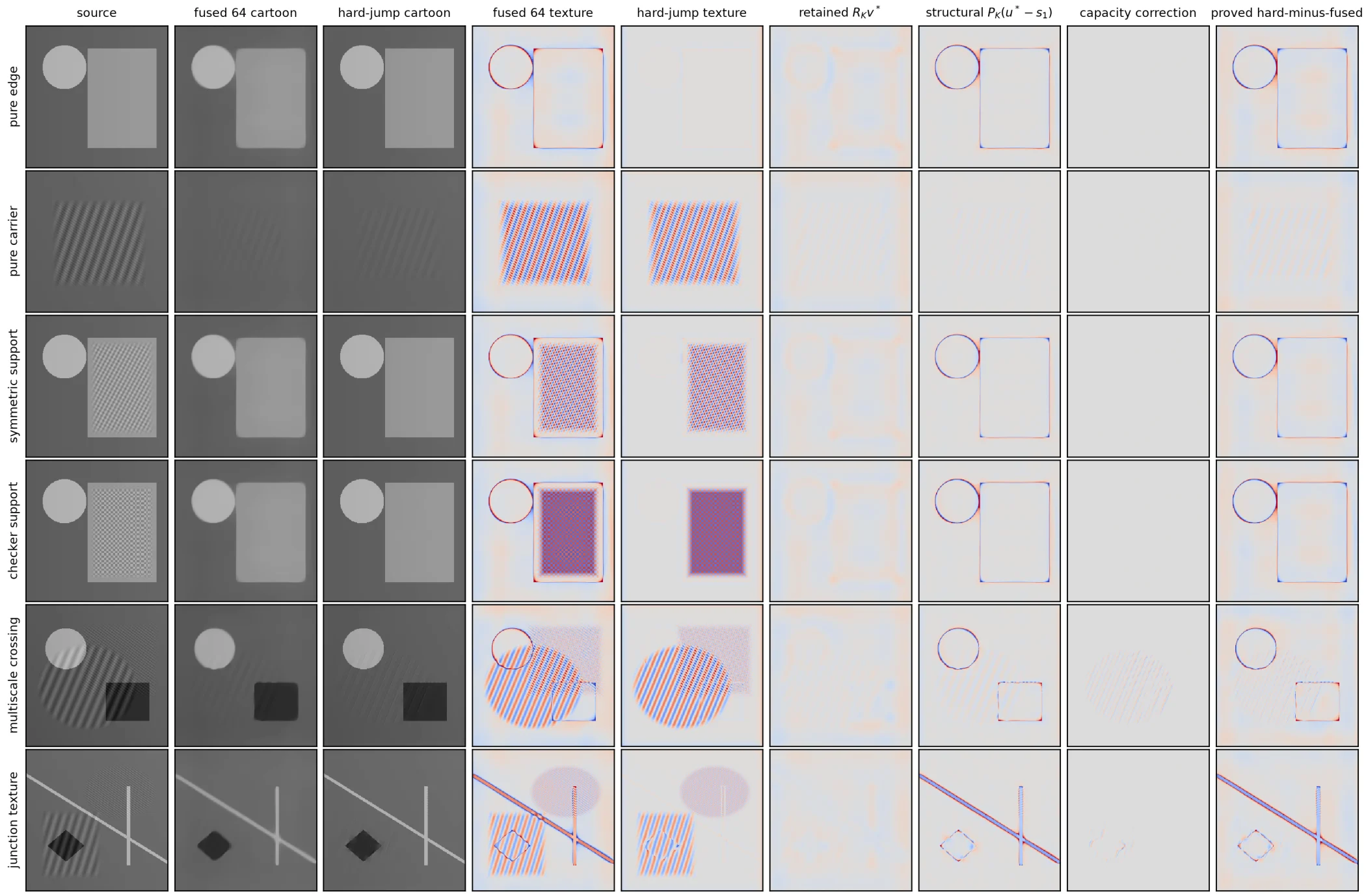
The rejected hard construction replaced a six-field nonlinear recurrence with two scalar observations. Against any exact two-product reference, its texture error separates algebraically into a structural high-pass, an uncompleted carrier tail, and the final capacity correction.

v_H − v_* = P_K(u_* − s₁) − H^Kv_* + q_μ P_K = I − H^K

The first term is the paired positive–negative contour response: a zero-mean halo created when a step mismatch is high-passed. The second is the carrier that no finite scalar contraction can finish. On six surgical controls, direct substitution leaves at most 1.42×10⁻¹³ in L∞.

The defect can be taken apart exactly.

Pure edge and pure carrier controls isolate the two terms; compound scenes show their superposition. The proved sum agrees with hard texture minus fused-64 texture to roundoff.

Six surgical controls decomposing the old hard-jump error into retained carrier, structural halo, capacity correction, and their proved sum — The last four columns are an identity, not a visual attribution: retained carrier + structural halo + capacity correction = hard texture − fused-64 texture.

The public cartoon is not the raw primal.

The optimized recurrence retains two primal fields and four accumulated gradient fields. At finite pass count, w = f − u − v is a survivor rather than disposable residue. Comparing raw u would therefore compare different objects.

The two-product output folds the survivor into the effective cartoon: v = f − u − w and ū = f − v = u + w. Every method shown on the page is displayed in this exact complementary coordinate.

cartoon primal

finite-pass survivor

t_xu

cartoon x accumulation

t_yu

cartoon y accumulation

t_xw

survivor x accumulation

t_yw

survivor y accumulation

Follow one finite-flow jump.

Select a station to inspect the fixed computation. There is no candidate scan, line search, classifier, learned threshold, or content-dependent branch.

Station 1 of 6

Enter the nonlinear chart.

Four ordinary fused passes establish a live primal–dual state before the first jump.

z ← T_f⁴(0)

The jump advances the recurrence already in use.

From the exact residual r = T_f(z) − z and a semismooth derivative A ∈ ∂T_f(z), the finite target is the polynomial displacement of the recurrence—not the stationary Newton solution.

p_m(A)r = (I + A + ··· + A^m−1)r

The implementation evaluates r, Ar, and A²r. A two-vector basis B = [r, Ar] reduces the Krylov projection to five deterministic inner products and a 2×2 polynomial. Short ordinary passes then refresh the disk-projection chart before the next jump.

FFT

source transform and ordinary prefix

one exact nonlinear residual

first streamed tangent pass

A²r

second streamed tangent pass

2×2

polynomial in registers

T_f²

two ordinary chart refreshes

The state jump removes the structural failure.

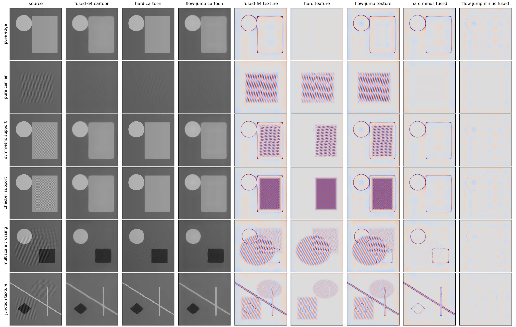
Across six controls, the old hard error retains its large contour and carrier pattern. The 29-cost quality schedule leaves a faint discrepancy with the character of ordinary finite convergence.

Six surgical controls comparing fused pass 64, the old hard jump, and the 29-cost finite-flow quality schedule — Fused-64 reference, rejected scalar hard jump, and finite-flow quality. The final two columns use a common diverging scale within each row.

Two fixed schedules move the quality frontier.

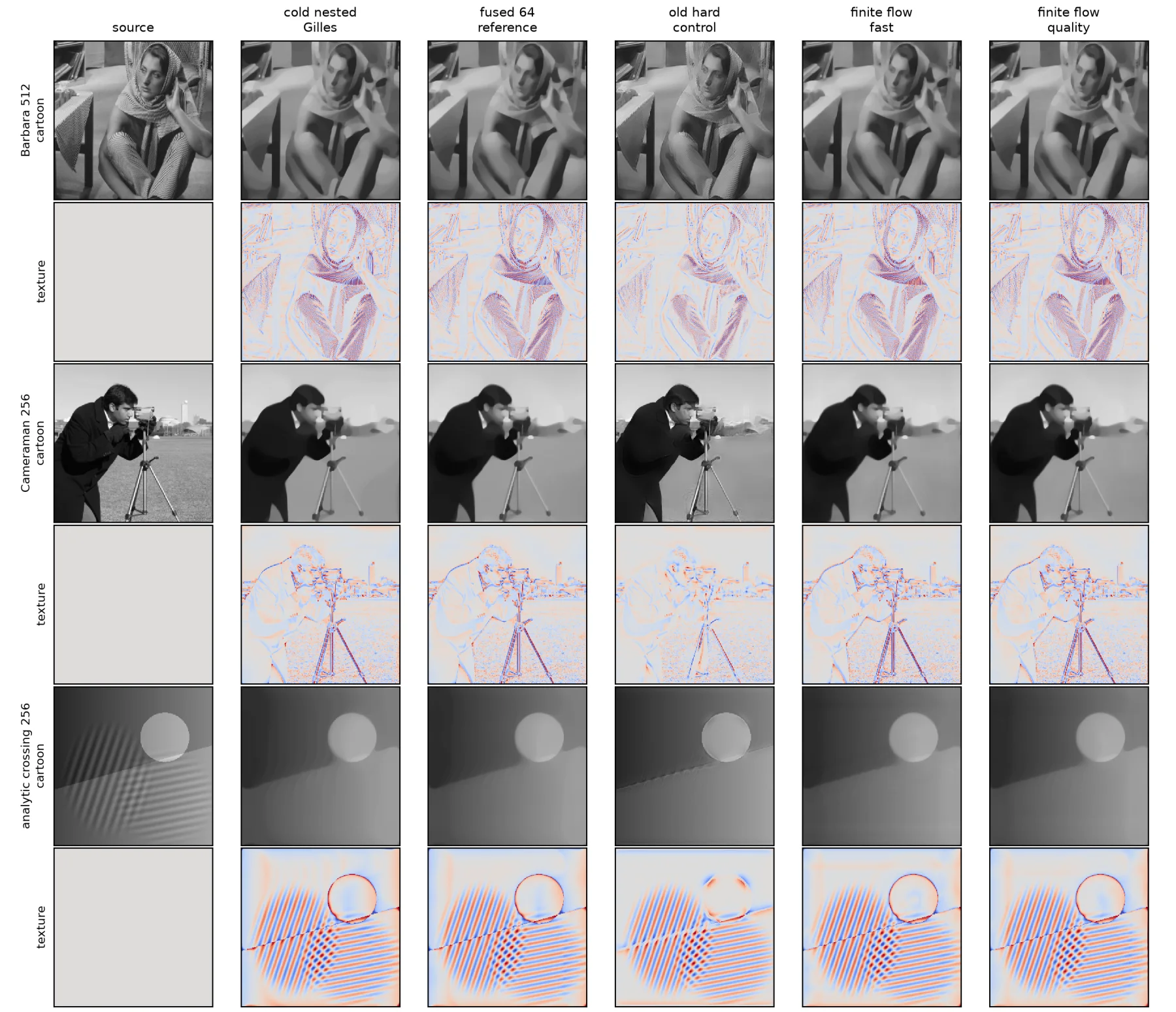
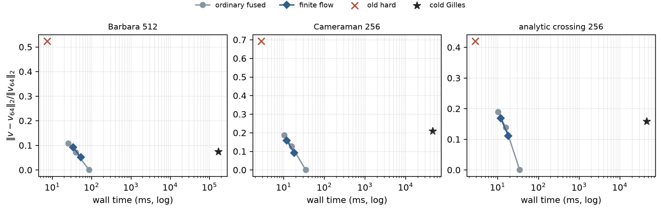
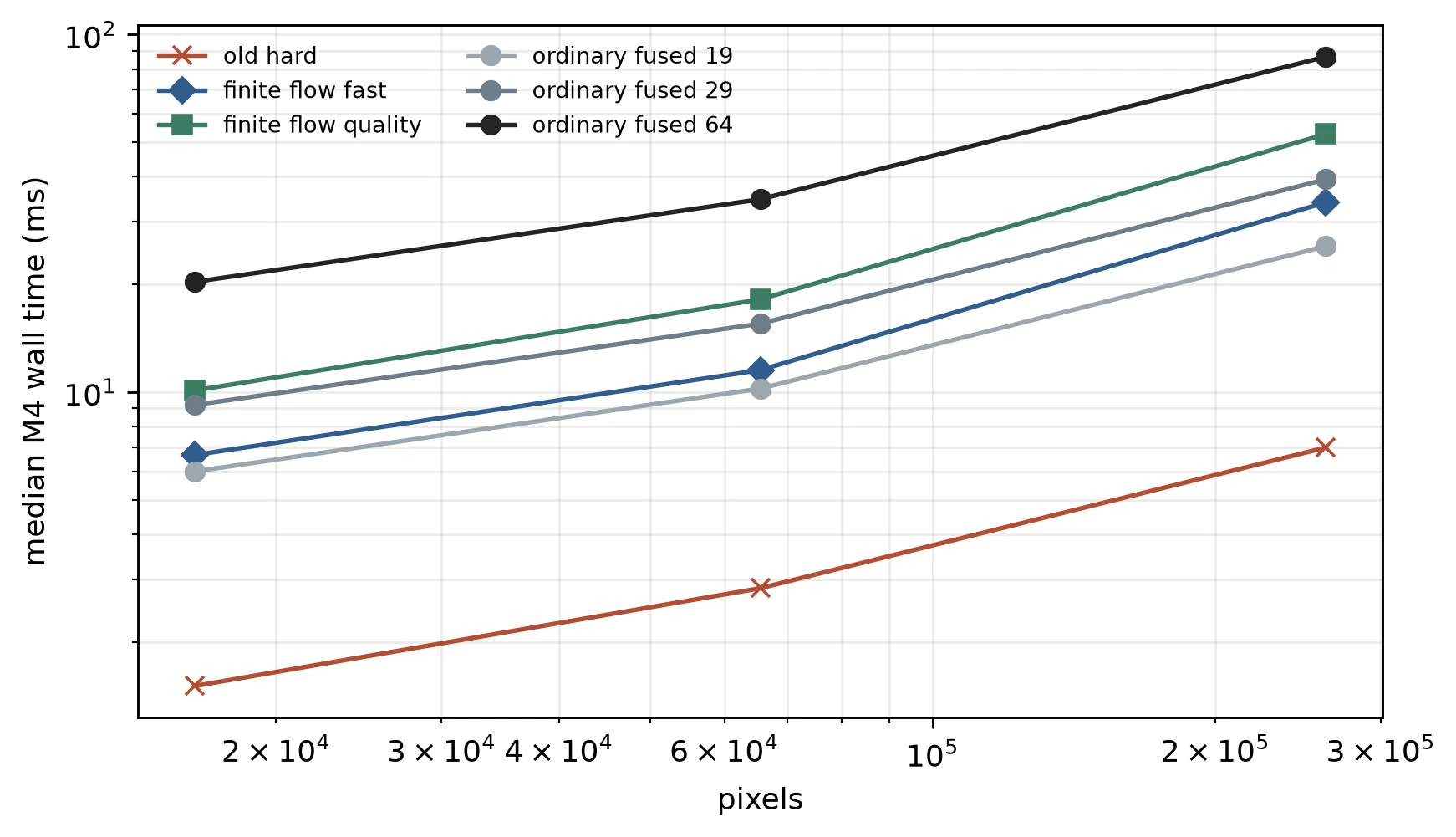
The fast schedule costs 19 operator passes; the quality schedule costs 29. Both are closer to fused pass 64 than ordinary fused iteration at the same operator cost on every surgical control and on Barbara, Cameraman, and an analytic crossing.

Finite flow fast

11.521 ms

Finite flow quality

18.155 ms

Fused pass 64

34.598 ms

256² · 8-thread M4 Mini

Measured schedule scaling

Fast speedup: 3.00×
Quality speedup: 1.91×
Fast operator cost: 19 passes
Quality operator cost: 29 passes

Medians after three warmups and eleven repeats; plan construction excluded. Schedule parameters are fixed independently of the source.

Natural and analytic comparison against fused pass 64
Method	Barbara 512²	Cameraman 256²	Analytic 256²
Old hard control	7.418 ms · E₆₄ .5235	2.821 ms · .6923	2.852 ms · .4200
Ordinary fused 19	25.583 ms · .1080	10.347 ms · .1863	10.182 ms · .1889
Finite flow fast	33.933 ms · .0923	11.959 ms · .1582	11.869 ms · .1689
Ordinary fused 29	39.545 ms · .0710	15.791 ms · .1273	15.849 ms · .1385
Finite flow quality	53.083 ms · .0513	18.144 ms · .0917	18.301 ms · .1111
Fused pass 64	86.988 ms · 0	34.864 ms · 0	34.732 ms · 0

Barbara, Cameraman, and analytic crossing comparisons across cold Gilles, fused 64, old hard control, and finite-flow fast and quality schedules — Exact two-product comparison. Fused pass 64 is the accepted trajectory reference; cold nested Gilles remains historical context, not ground truth.

Time-quality plots for Barbara, Cameraman, and analytic crossing comparing ordinary fused passes, finite-flow schedules, old hard control, and cold Gilles — The finite-flow diamonds improve on their equal-cost ordinary controls. Fused pass 64 defines zero reference error; the hard jump is fast but far from that accepted decomposition.

The claim is precise enough to fail.

Established here. The hard-jump error identity closes below 1.5×10⁻¹³ on six designed controls. Both fixed flow schedules beat equal-cost ordinary iteration across those controls and three comparison images.

Reference, not ground truth. Fused pass 64 is a finite, visually accepted trajectory target. Finite flow approximates that trajectory; it is not a theorem of BV/G uniqueness and does not equal a cold nested Gilles state.

Current boundary. Evidence covers λ=.05, μ=40, periodic full-spectral power-of-two shapes, six controls, and three comparisons. FACR and Neumann paths remain ordinary fused methods.

The implementation exposes the trade directly.

The full-spectral entry point is bfft_meyer_split_flow_jump; Python exposes MeyerPlan.split_flow_jump. The default full-spectral split uses the quality schedule, while the video demo uses fast. FACR plans keep their configured ordinary fused recurrence because the present tangent is full-spectral.

Native M4 wall-time scaling for old hard, finite-flow fast and quality, and ordinary fused 19, 29, and 64 schedules at 128, 256, and 512 square — Native scaling on an 8-thread M4 Mini. At 512², fast is 2.55× and quality is 1.64× faster than fused pass 64.

Read the proof or run the state jump.

The revised paper contains the recurrence, exact defect identity, semismooth finite-flow derivation, schedules, ablations, measurements, scope, and reproduction paths. The repository contains the C++ operator, Python binding, demos, proof arrays, and tests.